Dilated Convolutions for Modeling Long-Distance Genomic Dependencies

Tuesday. October 03, 2017

Gupta, A. and Rush, A.M., 2017. Dilated Convolutions for Modeling Long-Distance Genomic Dependencies. arXiv preprint arXiv:1710.01278

This blog post motivates and summarizes the paper (citation above) that I presented at ICML 2017 in August. I was invited to give a talk at the workshop, and also won a speaker award and best paper award at the conference. Read the paper on arXiv. There is a rough version of the code available on Github, and we will soon be releasing a much better and easy-to-use version.

I also want to give a special thanks to Dave Kelley, now at Calico, who was a helpful guide for understanding the complexity of this domain.

Overview of Machine Learning \(\times\) Genomics

In the past few years, there have been significant advances in both machine learning and genomics. In machine learning, there has been rapid advancement on tasks like image classification, segmentation, and machine translation using deep neural networks. These models require large amounts of training data, and put simply usually either learn hierarchical features through convolutional layers or sequential dependencies through recurrent layers.

At the same time, there has been a dramatic change in the study of the human genome. In the early 2000s, the Human Genome Project had just published its initial results, and researchers were only just beginning to get their hands on large-scale genomic data. Now, entire genomes can be sequenced cheaply, and techniques like ChipSeq and Hi-C have enabled researchers to get cell-type specific genome-wide characterizations of regulatory activity.

With these experimental techniques has come a massive range of curated raw data sources, containing information like the locations of transcription factor binding sites, histone modifications, and DNAse hypersensitivity sites. The availability of this data leads to a series of questions: can we use machine learning to model the regulatory regions of the genome? Moreover, to what extent do methods that were originally developed for images and text apply to genomic data? Does a new class of methods need to be developed?

Problem Motivation

One of the defining aspects of human DNA is its complex structure. Since grade school, we are taught to visualize DNA as the Watson and Crick style double helix: a pair of linear strands winding around one another. While this characterization is easy to understand, we now know that the genome is much more complicated. This “linear” strand is actually tightly compacted in 3-dimensional space, meaning that DNA locations that are far apart along the 1-dimensional sequence may be adjacent and able to interact. The nature of this compacting is thought to be regulated by a variety of factors, including chemical modifications to bound proteins called histones and the binding of external proteins called transcription factors. In the figure below, you can see how the DNA bends, which makes distal motifs coexist spatially.

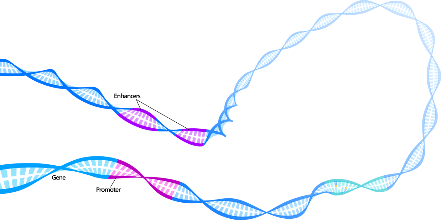
Thus, if we are trying to predict the locations of regulatory markers directly from a DNA sequence, it follows that capturing information across a very wide strand of DNA should improve accuracy. In machine learning, we formally refer to this property as receptive field size. The receptive field of an output neuron in a neural network is the set of inputs that affects it. Thus, we wish to build a model with large receptive fields. In order to naively scale existing approaches for regulatory marker prediction to larger receptive fields, the models would require a linear increase in the number of parameters, which makes them prone to overfitting and reduces training speed. Moreover, usually effective recurrent neural network models such as LSTM-based networks are difficult to train due to the long sequence lengths.

Solution: Dilated Convolutions

To address this challenge, we need a model in which the number of parameters grows sublinearly with respect to the input size, and in which we can parallelize our predictions across the input sequence (as it may be very long). The first constraint makes standard convolutional neural networks impractical, as their parameters grow linearly with respect to the receptive field of a given output. The latter constraint makes standard LSTM-based networks impractical too.

Instead, we use a dilated convolutional neural network. The receptive field size of a dilated CNN is exponential in the number of layers. This means that we can scale our models to several orders of magnitude more inputs than existing approaches, while only requiring a small increase in the number of parameters. Moreover, since these are adaptations of convolutions, we can implement these in a highly-parallelizable manner on GPU hardware in standard neural network packages. Dilated convolutions are best understood visually: below, see a comparison between the receptive fields of standard CNNs, recurrent neural networks, and dilated convolutions.

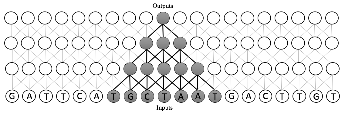
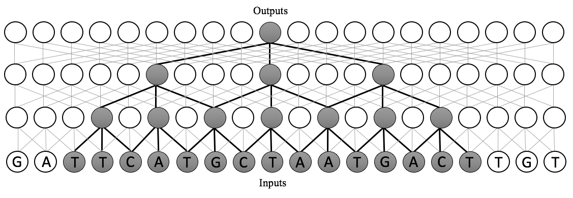
In short, a dilated convolution is a generalization of a standard convolution in which the inputs are dilated, or spaced, by some predefined dilation rate. A dilated convolution with dilation rate 1 is a standard convolution. With dilation width \(d\), the window starting at location \(i\) of size \(k\) is

\[\begin{bmatrix} \mathbf{x}_i & \mathbf{x}_{i + d} & \mathbf{x}_{i + 2d} & \cdots & \mathbf{x}_{i + (k-1)\cdot d} \end{bmatrix}\]

By increasing the dilation rate exponentially as we go up the layers, we get a receptive field that is exponential in the number of layers.

Dataset and Problem Statement

After establishing the baseline performance of our model on an existing dataset, we tested the ability to learn long-term dependencies. The rest of this blog post will focus on our dataset and the results on it, but to see the details of the baseline, check out the full paper.

In order to model long-distance dependencies, we introduce a new dataset that uses the same raw data sources as existing work. However, it has two major differences from past work:

1. The input sequences are longer, with each a 25,000 bp sequence (vs 1000 bp).
2. The outputs annotate at nucleotide resolution, making this a dense labeling task. We predict the presence of all regulatory markers at each nucleotide, rather than once per sequence.

Thus, in this setup, we have a dataset \(D\) with pairs of input/output sequences

\[D = \{(\mathbf{x}, \mathbf{y})\}\]

with \(\mathbf{x} \in V^d\), \(\mathbf{y} \in \{0, 1\}^{d \times k}\), \(d = 25000\), and \(k = 919\).

We train several architectures on this model, including standard convolutional neural networks, bidirectional LSTMs, and dilated convolutional neural networks. We do extensive hyper parameter sweeps with each of these models. Though there is definitely more principled work to be done in comparing these approaches thoroughly (and that is ongoing!), this gives us a rough set of baselines for each of these approaches. Please see the full paper for details about the hyperparameter tuning, model specifics, and more.

Results:

Model	Layers	Type	Params	Validation PR AUC			Test PR AUC
				TFBS	Hist	DNAse	TFBS	Hist	DNAse
CNN7	7	CNN	656363	0.167	0.166	0.180	0.167	0.165	0.186
Bi-LSTM	4	Bi-LSTM	764395	0.104	0.288	0.116	0.107	0.264	0.113
Dilated	6	Dilated Conv	631263	0.274	0.279	0.178	0.274	0.273	0.179

Dilated convolutional models perform the best on both TFBS and histone modification prediction, and do marginally worse than the best non-dilated models on predicting DNAse hypersensitivity sites. This shows that dilated convolutions can be effective at capturing genome structure. We also note that the bidirectional LSTM does much worse than the dilated convolution across the board, consistent with the difficulty in training LSTMs across very long sequences.

On DNAse hypersensitivity prediction, we actually find that standard deep convolutions do well. This may be because accessible regions have highly explanatory local motifs, and having additional context far away does not improve the accuracy, which makes sense since accessible regions tend to be where binding activity occurs, and thus where we may expect to detect binding motifs. However, the other two marker types are more easily characterized with access to distal regions.

Visualizing the Receptive Fields

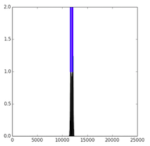
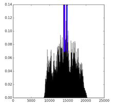
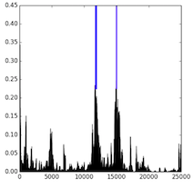
To further investigate the trained models, we visualize the receptive fields by sampling a validation sequence and backpropagating an error of 1 from every positive output for a random regulatory marker. We plot the output locations (blue) and the norm of the error to the inputs (black), which gives a visual of the receptive field. Here, we see that the standard convolution has a narrow receptive field, while the dilated convolution has a wide one. In contrast, while the LSTM has a wide receptive field, we can see that the magnitude of the gradient is low to most of the input. In does not appear that the LSTM models are able to learn the long-distance depdencies that the dilated model captures.

CNN7	Dilated	Bi-LSTM

Future Work

There are several avenues for future work in this space. First, we use two datasets to do our implementation, one was an existing baseline that used 1000bp to classify the whole sequence, and the other was our new dataset that uses 25000 bp and then labels the whole sequence. These are different tasks, and as such their results cannot be directly compared. As such, we intend to also implement 1000 bp labeling and 25000 bp classification, which would allow us to more thoroughly determine the extent to which these architectures are effective in different domains.

We have other ideas about incorporating transcription factor amino acid sequences, predicting methylation, and building more coherent datasets that address multiple tasks at once. If you have any ideas about any of these or want to collaborate, please reach out.